Overview
I’ve recently started using Snowflake for work. I’m keen to enable more active use of geospatial data, and so I’ve been weighing up the merits of using something like Snowflake rather than, say, PostGIS. Snowflake is lacking in features compared to PostGIS–it has far fewer spatial functions, and a particular issue for me is the lack of support for any geodetic datum other than WGS84. On the other hand, if most of your other data will be stored in Snowflake, then having it all in one place greatly enhances the ability to mash things up in-place.
As part of my exploration, one thing I found particularly niggly was the load process itself. It is relatively easy to load data into PostGIS from a variety of data sources, either using the ogr2ogr tool provided as part of the GDAL suite; or utilities provided by PostGIS itself, such as shp2pgsql. By contrast, I’d found loading spatial data to Snowflake significantly less straightforward. I understand that FME Workbench can handle the job, but I don’t have access to it currently where I work, and don’t think I’d use it enough to justify its procurement.
Curiously, my first attempt (which worked rather well), involved PostGIS. I’d first load a feature class to PostGIS, then I’d dump the results of a query into a CSV file, where I’d replace the geometry with well-known text (WKT) using the ST_AS_TEXT function. When copying data from CSV, Snowflake will happily convert WKT to its own GEOGRAPHY type if that’s what the schema demands, and so the method is effective enough. However, if exploring the use of Snowflake as an alternative to PostGIS, it does seem peculiar to involve PostGIS as part of the load process.
As an alternative, we can use either of the ODBC or JDBC drivers to insert records. We just need to find a client library or wrapper that we’re comfortable with. I found an approach using R which is both easy and performant, and so I thought it would be worth describing. The post will be brief, but hopefully useful to somebody.
Our Task
We’ll simply create a schema in a Snowflake database called GIS, and then we’ll load a reasonably large feature class into a table. We’ll use New Zealand building outlines extracted from OpenStreetMap. A New Zealand extract can be downloaded directly from:
Geofabrik Download Server - New Zealand
This contains 18 or so feature classes, including land use and places of interest, but we’ll consider specifically the shapefile named gis_osm_buildings_a_free_1. This is about 500MB on disk, and contains nearly 1.5 million outlines.
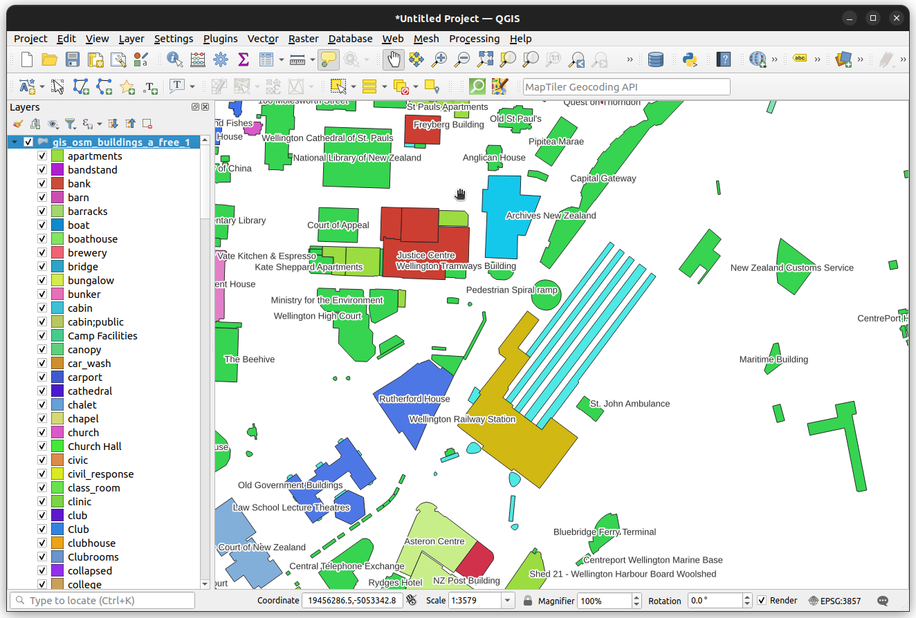
openstreetmaps building outlines, coloured by fclass.
Requirements
The primary requirement will simply be a recent version of R, and the sf package. In addition, we will also choose to do basic manipulation using the data.table package. We will need additional packages, and the specifics will depend whether we are using the ODBC or JDBC drivers.
ODBC
If using ODBC, R users will need to install the odbc package, as well as the Snowflake ODBC driver. See:
JDBC
If using JDBC, R users will need to install the RJDBC package. This depends in turn on the rJava package, and a usable Java Development Kit will need to be present for this to work correctly. Otherwise, users simply need to download the JDBC driver. This can be fetched directly from Maven, for example via:
The ODBC driver will probably be a little faster than the JDBC driver. In saying that, if you work in a Windows environment, the ODBC driver will need to be installed via an MSI file, and this might require some effort in some enterprise settings. On the other hand, the JDBC driver has no such requirement, and is easy enough to use if you already have access to a functioning JDK.
Let’s Do It…
We first need to establish a database connection. If using ODBC, this will look something like:
con <- DBI::dbConnect(
  odbc::odbc(),
  .connection_string = "
  Driver=SnowflakeDSIIDriver;
  server=<server>.<location>.snowflakecomputing.com;
  uid=<user ID>;
  authenticator=externalbrowser;
  database=<database>;
  warehouse=<warehouse>;
  tracing=2;
  "
)
If using JDBC, this will look something like this:
library(RJDBC)

# I like to define an infix operator for concatenating strings...
`%+%` <- function(a, b) sprintf("%s%s", a, b)

# create the driver
drv <- JDBC(
  "net.snowflake.client.jdbc.SnowflakeDriver",
  "./inst/java/snowflake-jdbc-3.13.17.jar"
)

# create connection string
constr <- sprintf(
  "jdbc:snowflake://%s.snowflakecomputing.com/?" %+%
    "db=%s&wharehouse=%s&user=%s&authenticator=externalbrowser",
  "<account>.<location>",
  "<database>",
  "<warehouse>",
  "<user ID>"
)

# create connection
con <- DBI::dbConnect(drv, constr)
We then create our GIS schema:
DBI::dbSendQuery(con, "CREATE SCHEMA IF NOT EXISTS GIS")We will also need to create an empty table to hold our features:
create_query <- "
CREATE TABLE GIS.OSM_BUILDINGS_A_FREE_1 (
  OSM_ID VARCHAR PRIMARY KEY,
  CODE INTEGER,
  FCLASS VARCHAR,
  NAME VARCHAR,
  TYPE VARCHAR,
  GEOMETRY GEOGRAPHY
)
"

DBI::dbSendQuery(con, create_query)
We then import our shapefile as follows:
buildings <-st_read("data-raw/osm/gis_osm_buildings_a_free_1.shp")We know the geometry column is called geometry since this is the value of the the sf_column attribute:
attr(buildings, 'sf_column')[1] "geometry"Now we simply convert to data.table, and replace the geometry column with the well-known binary representation:
buildings[, geometry := st_as_binary(geometry, hex = TRUE, pureR = FALSE)]On my machine with with i7-950H (12) processor, this took 9.7 seconds. This object is about 1.3GB in-memory and contains nearly 1.5 million features, so this is pretty quick. In my first attempt at this, I tried to extract well-known text (WKT), as opposed to binary, using st_as_text, and this same step took around 20 minutes!!
All we need to do now is upper-case the column names to match our target schema, and we can then load our table directly:
setNames(buildings, colnames(buildings), toupper(colnames(buildings)))When attempting to load the data in one go I received a memory allocation error. I didn’t look into this in much detail, and simply decided to load the data in chunks. To do this:
lo <- seq(1, nrow(buildings), 10000)
hi <- c(lo[-1] - 1, nrow(buildings))

for (i in 1:length(lo)) {
  DBI::dbAppendTable(
    con,
    DBI::Id(schema = "GIS", table = "OSM_BUILDINGS_A_FREE_1"),
    buildings[lo[i]:hi[i],]
  )
}
This took 11 minutes for me overall. We had 146 lots of 10000, and the Snowflake logs suggest that each of these took about 2 seconds. So, about 6 minutes was spend loading data, with the balance, around 5 minutes, being spent transferring the data over the wire. Overall, I’m pretty happy with this from a performance perspective, and it would be easy enough to turn what we showed here into something a bit more generic. Either way, until such time as a Snowflake driver is added to GDAL, this will do fine.